R Code

news
code
analysis
Author

川口淳

Published

2026-09-03

本書で使用したRコードを共有します。

二値データと二項分布

## ==== パラメータ設定 ====
set.seed(123)
p <- 0.4       # 母比率
n <- 6          # 標本サイズ
B <- 10000      # シミュレーション回数

## ==== シミュレーション ====
x <- rbinom(B, size = n, prob = p)

## ==== 集計(有病者数・標本比率・度数)====
k_vals <- 0:n
freq   <- tabulate(x + 1, nbins = n + 1)

res <- data.frame(有病者数 = k_vals, 標本比率 = round(k_vals / n, 2), 度数 = as.integer(freq),
  row.names = NULL, check.names = FALSE
)
res
  有病者数 標本比率 度数
1        0     0.00  487
2        1     0.17 1835
3        2     0.33 3169
4        3     0.50 2766
5        4     0.67 1369
6        5     0.83  336
7        6     1.00   38

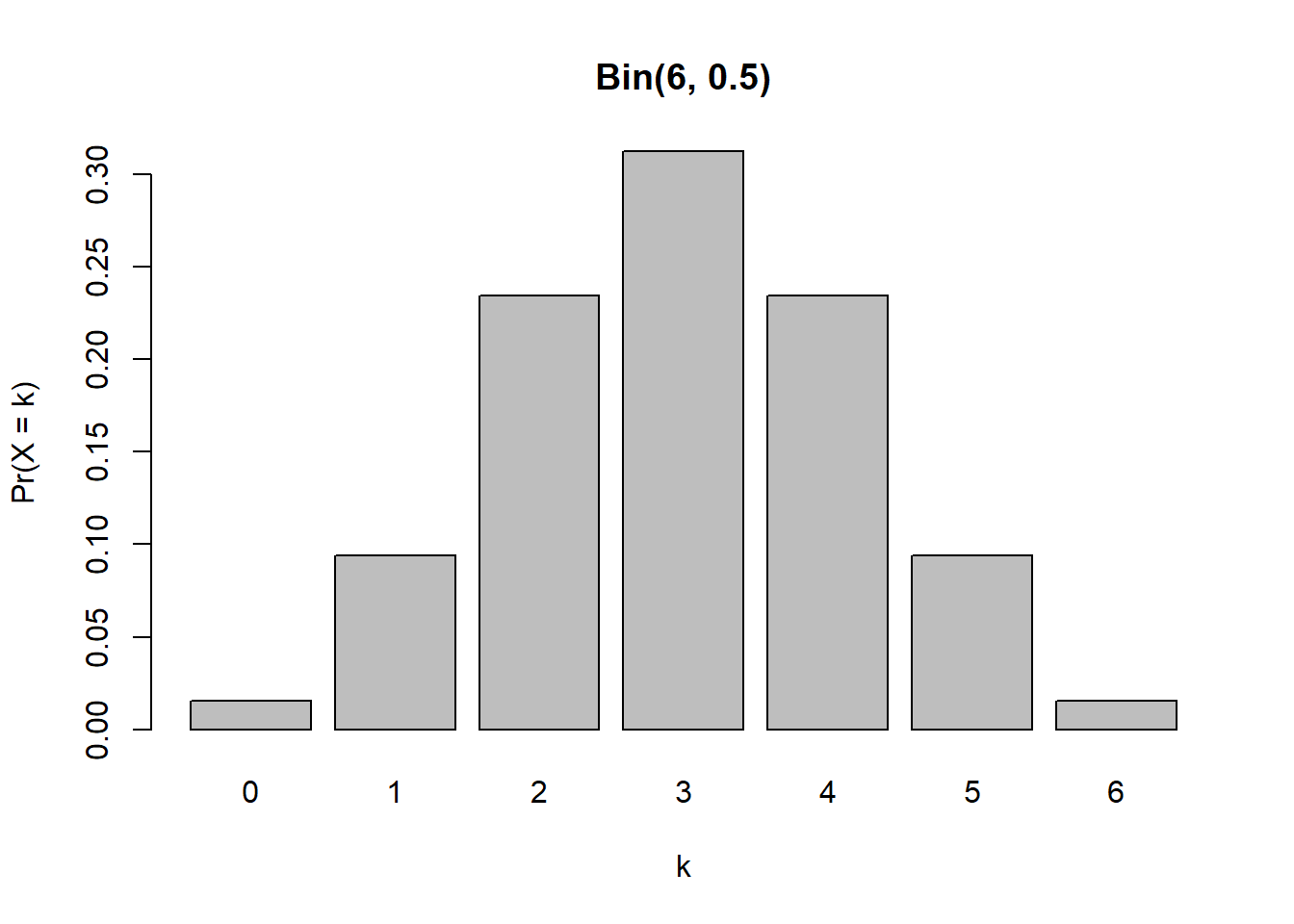
二項分布の図示

x <- 0:6
barplot(dbinom(x, size = 6, prob = 0.5),
  names.arg = x, main = "Bin(6, 0.5)", xlab = "k", ylab = "Pr(X = k)"
)

連続データと正規分布

例3.1:身長データ (70ページ)

\(\operatorname{Pr}(Z \leq 0.8)\)を求める.

pnorm(0.8)
[1] 0.7881446

\(\operatorname{Pr}(Z \leq-1.2)\)を求める.

pnorm(-1.2)
[1] 0.1150697

\(\operatorname{Pr}(Z \leq 0.8)-\operatorname{Pr}(Z \leq-1.2)\)を求める.

pnorm(0.8) - pnorm(-1.2)
[1] 0.6730749

標準化しないで計算する.

pnorm(120, 116, 5) - pnorm(110, 116, 5)
[1] 0.6730749

割合の推定と検定

80ページ

# 例:n=10, p=0.5, 観測値 x=1
n     <- 10
p     <- 0.7
x_obs <- 4

# $p$値(片側:X <= x_obs)
(p_value <- pbinom(x_obs, size = n, prob = p))
[1] 0.04734899

84ページ

# 正規近似による$p$値(連続性補正あり)
mu <- n * p
sigma <- sqrt(n * p * (1 - p))
(p_norm <- pnorm(x_obs + 0.5, mean = mu, sd = sigma))  # +0.5 は連続性補正
[1] 0.04224897

例4.2:母比率の検定(88ページ)

# ---- 設定 ----
x  <- 45        # 試行回数
n  <- 100         # 各試行の標本数

# ---- 95%信頼区間----
prop.test(x, n, conf.level = 0.95, correct = FALSE)

    1-sample proportions test without continuity correction

data:  x out of n, null probability 0.5
X-squared = 1, df = 1, p-value = 0.3173
alternative hypothesis: true p is not equal to 0.5
95 percent confidence interval:
 0.3561454 0.5475540
sample estimates:
   p 
0.45 

平均の推定と検定

例5.2:血清総コレステロールの平均(103ページ)

(Z = (204 - 200)/(40/sqrt(400)))
[1] 2
2*(1-pnorm(Z))
[1] 0.04550026

例5.3:コレステロールの例2(131ページ)

mu0 = 200
mu1 = 210
sigma = 40

(d = sigma / (mu1 - mu0))
[1] 4
alpha = 0.05
beta = 0.2
(zalpha = qnorm(1-alpha))
[1] 1.644854
(zbeta = qnorm(beta))
[1] -0.8416212
(n = (d * (zalpha - zbeta))^2)
[1] 98.92092
#切り上げ
ceiling(n)
[1] 99

群間比較

例6.1:2群の血圧変化量の差(142ページ)

※ 途中計算における四捨五入の影響で数値は完全には一致しません.

fname1 = "../data/2群の血圧変化量の差.xlsx"
sheetnames = readxl::excel_sheets(fname1)
(df = readxl::read_xlsx(fname1, sheet = 1))
# A tibble: 9 × 3
  id    group  delta
  <chr> <chr>  <dbl>
1 I1    介入群    -2
2 I2    介入群    -6
3 I3    介入群    -3
4 I4    介入群    -1
5 I5    介入群    -5
6 C1    対照群     2
7 C2    対照群    -1
8 C3    対照群     0
9 C4    対照群    -2
# ===== $t$検定(等分散を仮定) =====
t.test(delta ~ group, data = df, var.equal = TRUE)

    Two Sample t-test

data:  delta by group
t = -2.4388, df = 7, p-value = 0.04483
alternative hypothesis: true difference in means between group 介入群 and group 対照群 is not equal to 0
95 percent confidence interval:
 -6.20413379 -0.09586621
sample estimates:
mean in group 介入群 mean in group 対照群 
               -3.40                -0.25 

例6.2:2群の割合の差(151ページ)

(tb <- matrix(c(56, 24, 40, 40), nrow=2, byrow=TRUE, dimnames=list(群=c("新規治療群","標準治療群"), 転帰=c("奏効あり","奏効なし"))))
            転帰
群          奏効あり 奏効なし
  新規治療群       56       24
  標準治療群       40       40
csm = colSums(tb)
rsm = rowSums(tb)
asm = sum(tb)
prop1 = prop.table(tb, margin=1)  # 群ごとの奏効率
pdif = prop1[1,1]-prop1[2,1]
r = csm[1] / asm
se = round(sqrt(r*(1-r)*(1/csm[1]+1/csm[2])),2)
Z = round(pdif / se,2)
p = round(2*(1-pnorm(Z)),4)
chi = round(Z^2,2)
pchi = round(1-pchisq(chi,1),4)
chisq.test(tb, correct=FALSE)  # カイ二乗検定(Yates補正なし)

    Pearson's Chi-squared test

data:  tb
X-squared = 6.6667, df = 1, p-value = 0.009823
chisq.test(tb, correct=TRUE)   # 参考:Yates補正あり

    Pearson's Chi-squared test with Yates' continuity correction

data:  tb
X-squared = 5.8594, df = 1, p-value = 0.01549

例6.3:2群のHbA1c 値の差(157ページ)

interv_vals  <- c(5.6, 5.7, 5.8, 6.0, 6.0)  
control_vals <- c(5.9, 6.1, 6.2, 6.3, 6.5, 10.0)

m=length(interv_vals); n=length(control_vals); N=m+n
m1=m*(N+1)/2; s1=sqrt(m*n*(N+1)/12)
(z=(17-30)/5.5)
[1] -2.363636
(p=2*(1-pnorm(abs(round(z,2)))))
[1] 0.01827494

回帰分析

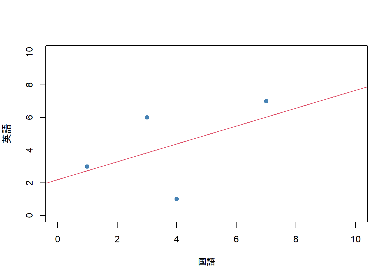
例7.1:国語と英語の点数(184ページ)

国語 = c(1, 3, 4, 7)
英語 = c(3, 6, 1, 7)

lmfit = lm(英語~国語)
summary(lmfit)

Call:
lm(formula = 英語 ~ 国語)

Residuals:
      1       2       3       4 
 0.2533  2.1600 -3.3867  0.9733 

Coefficients:
            Estimate Std. Error t value Pr(>|t|)
(Intercept)   2.2000     2.9280   0.751    0.531
国語          0.5467     0.6762   0.808    0.504

Residual standard error: 2.928 on 2 degrees of freedom
Multiple R-squared:  0.2463,    Adjusted R-squared:  -0.1305 
F-statistic: 0.6536 on 1 and 2 DF,  p-value: 0.5037
plot(英語~国語, xlab = "国語", ylab = "英語", xlim = c(0, 10), ylim = c(0, 10), pch = 19, col = "steelblue")
abline(lmfit, col=2)

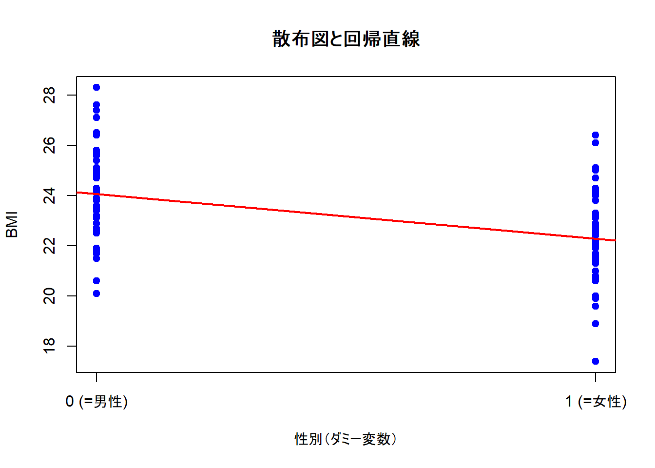
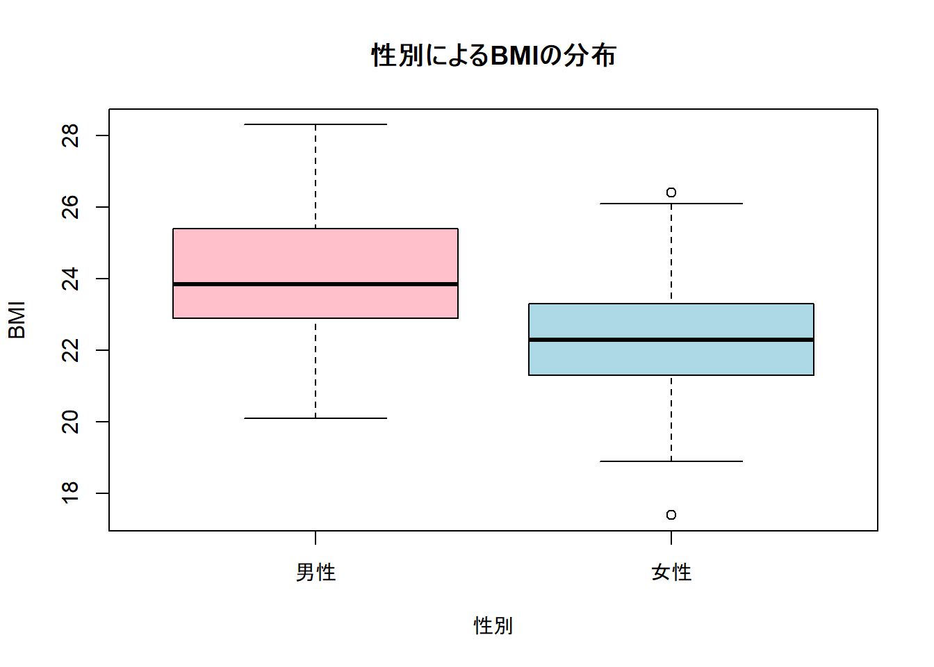
例7.2:BMI の性差(206ページ)

# 仮のデータ作成
set.seed(123)
gender <- factor(rep(c("男性", "女性"), each = 50), levels=c("男性", "女性"))
bmi <- round(c(rnorm(50, mean = 24, sd = 2), rnorm(50, mean = 22, sd = 2)),1)
data <- data.frame(gender, bmi)

gender_code <- ifelse(data$gender == "男性", 0, 1)

# 回帰モデル
model <- lm(data$bmi ~ gender_code)

# 左:散布図+回帰直線(横軸に0,1を表示)
plot(gender_code, data$bmi, xlab = "性別(ダミー変数)", ylab = "BMI", main = "散布図と回帰直線",
     xaxt = "n", pch = 19, col = "blue")
axis(1, at = c(0, 1), labels = c("0 (=男性)", "1 (=女性)"))  # 0,1を明示
abline(model, col = "red", lwd = 2)

# 右:箱ひげ図(女性を左、男性を右)
boxplot(data$bmi ~ data$gender, xlab = "性別", ylab = "BMI", main = "性別によるBMIの分布",
        col = c("pink", "lightblue"),
        at = c(1, 2)[order(levels(gender), decreasing = TRUE)])  # 順序逆転

# t検定による群間比較
t.test(bmi ~ gender, data = data, var.equal = TRUE)

    Two Sample t-test

data:  bmi by gender
t = 4.8528, df = 98, p-value = 4.594e-06
alternative hypothesis: true difference in means between group 男性 and group 女性 is not equal to 0
95 percent confidence interval:
 1.049736 2.502264
sample estimates:
mean in group 男性 mean in group 女性 
            24.068             22.292 
# 回帰分析(男性を基準)
fit <- lm(bmi ~ gender, data = data)
summary(fit)

Call:
lm(formula = bmi ~ gender, data = data)

Residuals:
   Min     1Q Median     3Q    Max 
-4.892 -1.168 -0.130  1.332  4.232 

Coefficients:
            Estimate Std. Error t value Pr(>|t|)    
(Intercept)  24.0680     0.2588  93.005  < 2e-16 ***
gender女性   -1.7760     0.3660  -4.853 4.59e-06 ***
---
Signif. codes:  0 '***' 0.001 '**' 0.01 '*' 0.05 '.' 0.1 ' ' 1

Residual standard error: 1.83 on 98 degrees of freedom
Multiple R-squared:  0.1937,    Adjusted R-squared:  0.1855 
F-statistic: 23.55 on 1 and 98 DF,  p-value: 4.594e-06

例7.3:血圧の変化量の群間差

fname1 = "../data/回帰分析例データ.xlsx"
dat = readxl::read_xlsx(fname1, sheet = 1)

## 平均差(試験群 − 対照群)と t検定
t.test(`血圧変化量` ~ 群, data = dat, var.equal=TRUE)  # t検定

    Two Sample t-test

data:  血圧変化量 by 群
t = -0.3356, df = 18, p-value = 0.7411
alternative hypothesis: true difference in means between group 試験群 and group 対照群 is not equal to 0
95 percent confidence interval:
 -7.986197  5.786197
sample estimates:
mean in group 試験群 mean in group 対照群 
               -15.1                -14.0 
summary(lm(`血圧変化量` ~ 群, data = dat))

Call:
lm(formula = 血圧変化量 ~ 群, data = dat)

Residuals:
    Min      1Q  Median      3Q     Max 
-10.900  -4.000  -0.900   2.775  14.000 

Coefficients:
            Estimate Std. Error t value Pr(>|t|)    
(Intercept)  -15.100      2.318  -6.515 3.99e-06 ***
群対照群       1.100      3.278   0.336    0.741    
---
Signif. codes:  0 '***' 0.001 '**' 0.01 '*' 0.05 '.' 0.1 ' ' 1

Residual standard error: 7.329 on 18 degrees of freedom
Multiple R-squared:  0.006218,  Adjusted R-squared:  -0.04899 
F-statistic: 0.1126 on 1 and 18 DF,  p-value: 0.7411
## ==== モデル設定(交互作用なし:平行な2本の回帰線) ====
fit <- lm(`血圧変化量` ~ 年齢 + 群, data = dat)
summary(fit)

Call:
lm(formula = 血圧変化量 ~ 年齢 + 群, data = dat)

Residuals:
    Min      1Q  Median      3Q     Max 
-3.9797 -1.7784 -0.4507  1.8272  3.8150 

Coefficients:
             Estimate Std. Error t value Pr(>|t|)    
(Intercept) -50.18002    2.97968 -16.841 4.87e-12 ***
年齢          0.57888    0.04752  12.181 8.00e-10 ***
群対照群      3.53129    1.09962   3.211  0.00512 ** 
---
Signif. codes:  0 '***' 0.001 '**' 0.01 '*' 0.05 '.' 0.1 ' ' 1

Residual standard error: 2.418 on 17 degrees of freedom
Multiple R-squared:  0.8978,    Adjusted R-squared:  0.8858 
F-statistic: 74.71 on 2 and 17 DF,  p-value: 3.791e-09

例7.4:有効率の群間差(225ページ)

# 2×2分割表データ(集計形式) 0=対照群, 1=新規群
df <- data.frame(群   = c(0, 1), 有効 = c(30, 45), 無効 = c(70, 55))

# 分割表の確認
tab <- rbind(
  新規群 = c(有効 = df$有効[df$群==1], 無効 = df$無効[df$群==1]),
  対照群 = c(有効 = df$有効[df$群==0], 無効 = df$無効[df$群==0])
)
tab
       有効 無効
新規群   45   55
対照群   30   70
# 粗オッズ比の手計算
odds1 <- df$有効[df$群==1] / df$無効[df$群==1]
odds0 <- df$有効[df$群==0] / df$無効[df$群==0]
(OR_crude <- odds1 / odds0)
[1] 1.909091
# ロジスティック回帰(集計二項データ):cbind(成功, 失敗)
fit <- glm(cbind(有効, 無効) ~ 群, family = binomial, data = df)
summary(fit)

Call:
glm(formula = cbind(有効, 無効) ~ 群, family = binomial, 
    data = df)

Coefficients:
            Estimate Std. Error z value Pr(>|z|)    
(Intercept)  -0.8473     0.2182  -3.883 0.000103 ***
群            0.6466     0.2967   2.179 0.029295 *  
---
Signif. codes:  0 '***' 0.001 '**' 0.01 '*' 0.05 '.' 0.1 ' ' 1

(Dispersion parameter for binomial family taken to be 1)

    Null deviance: 4.8247e+00  on 1  degrees of freedom
Residual deviance: 1.4433e-14  on 0  degrees of freedom
AIC: 13.94

Number of Fisher Scoring iterations: 3
coef(fit)       # a(切片), b(群の係数)
(Intercept)          群 
 -0.8472979   0.6466272 
exp(coef(fit))  # e^a(対照群のオッズ), e^b(オッズ比)
(Intercept)          群 
  0.4285714   1.9090909 

例7.5:重症度を考慮する合併症の群間差(234ページ)

table(dat$Y, dat$X)
   
      0   1
  0 283 232
  1  50  35
m_crude <- glm(Y ~ X, data=dat, family=binomial())
summary(m_crude)

Call:
glm(formula = Y ~ X, family = binomial(), data = dat)

Coefficients:
            Estimate Std. Error z value Pr(>|z|)    
(Intercept)  -1.7334     0.1534 -11.300   <2e-16 ***
X            -0.1580     0.2375  -0.665    0.506    
---
Signif. codes:  0 '***' 0.001 '**' 0.01 '*' 0.05 '.' 0.1 ' ' 1

(Dispersion parameter for binomial family taken to be 1)

    Null deviance: 489.57  on 599  degrees of freedom
Residual deviance: 489.13  on 598  degrees of freedom
AIC: 493.13

Number of Fisher Scoring iterations: 4
table(dat[dat$Z==0, "Y"], dat[dat$Z==0, "X"])
   
      0   1
  0 248  76
  1  29   4
table(dat[dat$Z==1, "Y"], dat[dat$Z==1, "X"])
   
      0   1
  0  35 156
  1  21  31
m_adj   <- glm(Y ~ X + Z, data=dat, family=binomial())
summary(m_adj)

Call:
glm(formula = Y ~ X + Z, family = binomial(), data = dat)

Coefficients:
            Estimate Std. Error z value Pr(>|z|)    
(Intercept)  -2.1196     0.1862 -11.382  < 2e-16 ***
X            -1.0250     0.2948  -3.477 0.000507 ***
Z             1.5554     0.2946   5.280 1.29e-07 ***
---
Signif. codes:  0 '***' 0.001 '**' 0.01 '*' 0.05 '.' 0.1 ' ' 1

(Dispersion parameter for binomial family taken to be 1)

    Null deviance: 489.57  on 599  degrees of freedom
Residual deviance: 459.79  on 597  degrees of freedom
AIC: 465.79

Number of Fisher Scoring iterations: 5

生存時間解析

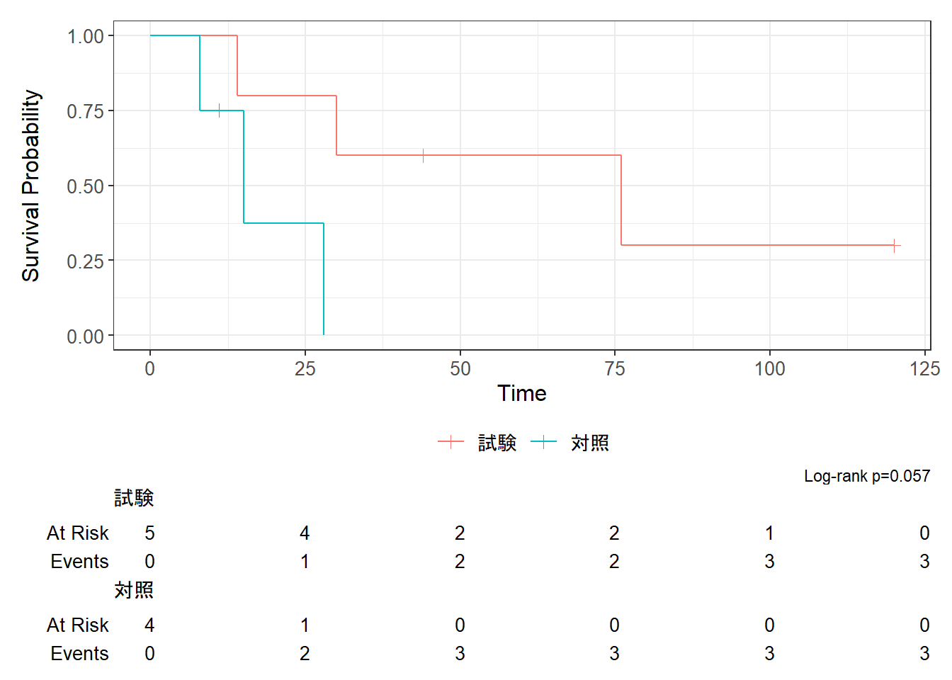
例8.2:2 群の生存時間データ(253ページ)

library(survival)
library(survminer)
Loading required package: ggplot2
Loading required package: ggpubr

Attaching package: 'survminer'
The following object is masked from 'package:survival':

    myeloma
library(ggsurvfit)

fname1 = "../data/生存時間例データ.xlsx"
survdata = readxl::read_xlsx(fname1, sheet = 1)

# 群別KM
(fit2 <- survfit2(Surv(生存時間, 打ち切り) ~ 群, data = survdata))
Call: survfit(formula = Surv(生存時間, 打ち切り) ~ 群, data = survdata)

        n events median 0.95LCL 0.95UCL
群=試験 5      3     76      30      NA
群=対照 4      3     15       8      NA
# ログランク検定
(lr  <- survdiff(Surv(生存時間, 打ち切り) ~ 群, data = survdata))
Call:
survdiff(formula = Surv(生存時間, 打ち切り) ~ 群, data = survdata)

        N Observed Expected (O-E)^2/E (O-E)^2/V
群=試験 5        3     4.74     0.637      3.62
群=対照 4        3     1.26     2.387      3.62

 Chisq= 3.6  on 1 degrees of freedom, p= 0.06 
# コンパクトなKM図
p = ggsurvfit(fit2) + add_risktable() + add_censor_mark() + add_pvalue(caption = "Log-rank {p.value}")
print(p)

例8.3:多変量の生存時間データ(265ページ)

# 全体ログランク
survdiff(Surv(time, status) ~ 治療群, data = dat)
Call:
survdiff(formula = Surv(time, status) ~ 治療群, data = dat)

             N Observed Expected (O-E)^2/E (O-E)^2/V
治療群=試験 59       49     57.8      1.35      3.47
治療群=対照 61       57     48.2      1.63      3.47

 Chisq= 3.5  on 1 degrees of freedom, p= 0.06 
# Cox(調整あり)
fit <- coxph(Surv(time, status) ~ 治療群 + 年齢 + 遺伝子, data = dat)
summary(fit)
Call:
coxph(formula = Surv(time, status) ~ 治療群 + 年齢 + 遺伝子, 
    data = dat)

  n= 120, number of events= 106 

              coef exp(coef) se(coef)     z Pr(>|z|)    
治療群対照 1.33997   3.81891  0.25173 5.323 1.02e-07 ***
年齢       0.02281   1.02307  0.01385 1.647   0.0996 .  
遺伝子陽性 1.89450   6.64921  0.26349 7.190 6.48e-13 ***
---
Signif. codes:  0 '***' 0.001 '**' 0.01 '*' 0.05 '.' 0.1 ' ' 1

           exp(coef) exp(-coef) lower .95 upper .95
治療群対照     3.819     0.2619    2.3317     6.255
年齢           1.023     0.9775    0.9957     1.051
遺伝子陽性     6.649     0.1504    3.9672    11.144

Concordance= 0.71  (se = 0.032 )
Likelihood ratio test= 57.24  on 3 df,   p=2e-12
Wald test            = 54.06  on 3 df,   p=1e-11
Score (logrank) test = 55.44  on 3 df,   p=6e-12